1.1
Narrowband
analysis
Narrowband frequency analysis is the recommended method of interpreting
vibration measurements in relation to the guidance limits or for investigation
purposes.
Narrowband frequency analysis should be capable
of resolving the frequency of individual components of interest over
the relevant frequency range.
1.2
Broadband
limits
Some guidance values based on broadband measurements of the
overall amplitude of composite frequency vibration are suggested in
later sections to simplify routine survey procedures.
Broadband
measurements should cover the specified range of vibration frequencies
for each particular application.
If the acceptability
of vibration severity is marginal from the results of broadband measurements,
narrow band frequency analysis should be used. Records of the vibration
measurements should be taken in such cases.
1.3
Orders of
vibration
Vibration frequencies can conveniently be related to a known
fundamental excitation frequency by the use of order numbers. In cases
where shaft rotational frequency is an appropriate reference, then:
Order numbers are typically integer numbers, 1, 2,
3,......,n. Vibration at four cycles per shaft revolution arising
from a four-bladed propeller, for example, can either be described
as occurring at shaft fourth order or at blade order. Half orders
(½, 1½, ...) may typically occur with 4-stroke diesel
engines where the working cycle takes place over two shaft revolutions.
1.4
Analysis
methods
Vibration data can be divided into two categories: steady and
transient. Some data with minimal transient characteristics can be
considered in a quasi-steady sense. The available analysis methods
are summarized in
Figure 3.1.1 Summary of available analysis methods
.
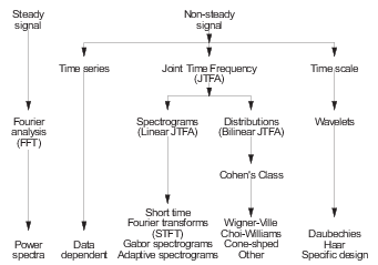
Figure 3.1.1 Summary of available analysis methods
1.5
Fast Fourier
Transform analysis
Analysis of steady and quasi-steady signals is usually carried
out using the Fast Fourier Transform (FFT) function found on most
vibration analysers.
An FFT analysis transforms consecutive
samples (typically 1024, 2048, or 4096) from the time domain to the
same number of lines in the frequency domain. The algorithm used to
calculate the FFT is finite and discrete. This has a number of effects.
The first is that aliasing might occur, when because of a limited
number of samples, high frequencies might appear as false lower frequencies.
This is avoided by lowpass “anti-aliasing” filters. A
sampling frequency higher than the maximum frequency of interest,
fmax , is used. This is determined by:
The frequency resolution is thus dependent on the
frequency range used, but most analysers have band- selectable analysis
which gives increased resolution or “zoom” at frequencies
of interest.
The second effect of a finite sample record
is that discontinuities can arise at the ends of the sample, giving
rise to false results when the signal is not periodic in the time
record. This causes leakage of energy from one resolution line of
the FFT into other lines. The amplitude at the start and end of each
block of samples is therefore reduced to zero, a technique known as
windowing. The Hanning window is a good, general purpose compromise
for continuous signals. A transient signal, such as from an impact,
is self-windowing and a Uniform (Rectangular) window should be used.
The third effect is known as the picket fence effect. It arises
from the discrete sampling of the spectrum in the frequency domain
in which the FFT acts like a series of parallel filters. The results
are similar to viewing the results through slits in a picket fence.
The shape or response of the filters is determined by the window
function used. The amplitude of a frequency which is in the middle
of a filter using a Hanning window will be measured accurately. A
frequency midway between filters could be attenuated by up to 1.5
dB (18%). The use of a Flat-top window will reduce the possible attenuation
to less than 0.1 dB (1%). However, the increase in accuracy comes
at the expense of frequency resolution of small components.
1.6
Time domain signal
It is desirable to view the “raw” vibration signal
(signal amplitude displayed against time) during analysis. Signal
characteristics such as beating, transients and irregularities can
be readily detected in the time domain. Approximate inspection methods
of analysis are recommended as a check on the results derived from
analytical techniques.
1.7
Averaging
Averaging is not always appropriate and its use may destroy
or disguise the original signal characteristics. This includes, for
example, signals arising from intermittent defects or averaging of
non-steady signals. It may be possible to use non-steady signal techniques
to give a better understanding of the signal characteristics. Root
mean square (r.m.s.) averaging will give a better estimate of the
value of a signal, but it will not improve the signal-to-noise ratio.
Linear averaging will improve the signal-to-noise ratio if a trigger
signal is available which is synchronous with the periodic part of
the signal.
1.8
Modulation
Modulation describes a time dependant variation, either random
or repetitive, in a vibration signal,
Figure 3.1.2 Vibration modulation
.
- Amplitude modulation arises, for example, in an eccentrically
mounted gear where the tooth meshing frequency is constant but the
amplitude varies, typically at once per revolution of the gear.
- Frequency modulation occurs, for example, in gears with tooth
spacing errors or the passing signal from torsionally vibrating gear
teeth.
- Phase modulation occurs, for example, onboard a twin screw ship
where the excitation varies in time.
These types of modulation can occur in the same signal, for
example in heavy weather where the speed and load of a ship’s
main engine may vary simultaneously or in the hunting of a governor
of an alternator set. Frequency analysis cannot describe the varying
amplitude and frequency. The information is interpreted as steady
sine waves which appear as side bands about the fundamental frequency.
The amplitude of the fundamental frequency may be significantly diminished
in cases of very heavy modulation.
One side effect of
modulation is that the ear may detect frequencies that do not exist
or may be outside the normal range of audible frequencies.
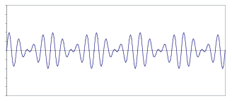
Figure 3.1.2 Vibration modulation
1.9
Rolling element
envelope analysis
Incipient defects in rolling element bearings produce sharp
pulses which may produce measurable frequencies up to 20 kHz. Identification
of the source cannot be carried out using simple FFT analysis and
a technique known as envelope analysis is used to extract useful information
from the vibration signal as follows. First the time domain signal
is band-pass filtered around the region of high frequency energy.
This leaves a signal containing bursts of energy at the defect frequency,
which is then rectified and low-pass-filtered. An FFT analysis of
the resultant signal will allow the defect frequency to be identified.
Calculation of the impact rates is given in
Table 3.1.1 Calculation of rolling element
impact frequencies
.
1.10
Calibration
Analysis methods should be verified using known input data.
Any software used in calibration, measurement or analysis should be
part of an appropriate Quality Assurance system.
Table 3.1.1 Calculation of rolling element
impact frequencies
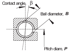
|
| Impact frequencies,
f Hz, assuming pure rolling:
|
|
|
Outer race defect,
|
|
|
|
Inner race defect,
|
|
|
|
Ball/ roller defect,
|
|
|
|
where
|
n = number of balls or rollers
|
|
|
|
fr
= relative revolutions per second between inner and outer races
|
|
|
|
B = ball or roller diameter
|
|
|
|
P = race pitch diameter
|
|
|
|
β = contact angle
|