
Section
3 Dynamic load components
3.1 Symbols
3.1.1 For the purposes of this Section, the following symbols apply:
 |
= |
wave coefficient to be taken as: |
| = |
0,0412L + 4,0 for L < 90 |
| = |
10,75 –  for 90 ≤ L ≤ 300 for 90 ≤ L ≤ 300 |
| = |
10,75 for 300 < L ≤ 350 |
| = |
10,75 –  for 350 < L ≤ 500 for 350 < L ≤ 500 |
 |
= |
1,2 for units without bilge keel |
| = |
1,0 for units with bilge keel |
 |
= |

,whichever is the greater, in metres
|
 |
= |
pitch radius and is to be taken as the greater of
 , in metres , in metres
|
 |
= |
 |
 |
= |
deep load draught, in metres |
 |
= |
draught in the loading condition being considered, in metres |
 |
= |
vertical acceleration due to heave, is to be taken as: |
| = |
 g m/s2 g m/s2
|
 |
= |
vertical acceleration due to pitch, is to be taken as: |
| = |
 m/s2 m/s2
|
 |
= |
vertical acceleration due to roll, is to be taken as: |
| = |
 m/s2 m/s2
|
 |
= |
transverse acceleration due to sway and yaw, is to be taken
as: |
| = |
0,3g
 m/s2 m/s2
|
 |
= |
transverse acceleration due to roll, is to be taken as: |
| = |
 m/s2 m/s2
|
 |
= |
longitudinal acceleration due to surge, is to be taken as: |
| = |
0,2g
a0 m/s2
|
 |
= |
longitudinal acceleration due to pitch, is to be taken as: |
| = |
 m/s2 m/s2
|
|
g |
= |
acceleration due to gravity, 9,81 m/s2
|
|
x |
= |
longitudinal coordinate of load point under consideration,
in metres |
|
y |
= |
transverse coordinate of load point under consideration, in
metres |
|
z |
= |
vertical coordinate of load point under consideration, in
metres |
 |
= |
longitudinal coordinate of reference point, for dynamic
tank pressures is to be taken as the middle of the tank length at the
top of the tank, in metres |
 |
= |
transverse coordinate of reference point, for dynamic tank
pressures is to be taken as the middle of the tank breadth at the top of
the tank, in metres |
 |
= |
vertical coordinate of reference point, for dynamic tank
pressures is to be taken as the highest point in the tank, in metres |
3.2 General
3.2.1
Basic components.
- Formulae for unit loads, motions and accelerations are given in
this sub-Section. Values calculated in accordance with the LR ShipRight
Procedure for Ship Units may be used instead.
- Formulae for the envelope value of the basic dynamic load
components are also given. The basic load components are:
- vertical wave bending moment and shear force;
- horizontal wave bending moment;
- dynamic wave pressure;
- dynamic tank pressures.
3.2.3
Metacentric height and roll radius of gyration for FPSO.
- The metacentric height, GM, and roll
radius of gyration,
 , should be calculated for typical loading conditions as
indicated in Table 2.3.1 GM and kr. For the initial
design of units storing oil in bulk (e.g. FPSOs), the values in Table 2.3.1 GM and kr may be used. The
values in Table 2.3.1 GM and kr for deep draught
condition may be used for the initial design of units for the flooded load
scenario, see
Pt 10, Ch 2, 5.1 Flooded condition. , should be calculated for typical loading conditions as
indicated in Table 2.3.1 GM and kr. For the initial
design of units storing oil in bulk (e.g. FPSOs), the values in Table 2.3.1 GM and kr may be used. The
values in Table 2.3.1 GM and kr for deep draught
condition may be used for the initial design of units for the flooded load
scenario, see
Pt 10, Ch 2, 5.1 Flooded condition.
3.3 Environmental factors
3.3.1 The environmental factors are used to derive the dynamic load components
for the intended site-specific condition and for the transit condition.
3.3.3 The environmental factors for the operational condition may be used for
the inspection/maintenance case. The environmental factors for the deep draught for
the operational condition may be used for the flooded case.
3.4 Return periods and probability factor,
fprob
3.4.2 In no case are the environmental loads used for the assessment of the
hull structure for on-site operation, restricted service area transit and delivery
voyage to be less than 50 per cent of the 25-year return period dynamic loads
defined for unrestricted worldwide transit service.
3.4.3 Environmental loads derived for the same wave environment, but at a
different return period, may be adjusted to the required return period by use of the
probability factor  . Therefore, when the environmental loads are derived for the
return periods specified in Table 2.3.3 Return periods for scantling
requirements and strength assessment, . Therefore, when the environmental loads are derived for the
return periods specified in Table 2.3.3 Return periods for scantling
requirements and strength assessment,  is to be taken as equal to 1. Probability factors should be
derived in accordance with the LR ShipRight Procedure for Ship Units. is to be taken as equal to 1. Probability factors should be
derived in accordance with the LR ShipRight Procedure for Ship Units.
3.4.4 The site-specific environmental factors, given in Table 2.3.2 Environmental factors, give 100-year return
period loads for the locations specified using all-year wave data. Therefore, when
using these factors for the on-site operation condition,  is to be taken as equal to 1. is to be taken as equal to 1.
3.4.5 At the request of the Owner and when consistent with the operational
philosophy of the unit, seasonal environmental data may be used to derive the
environmental loads for the inspection/maintenance condition. Alternatively, the
all-year loads derived for the on-site operation condition may be used for the
inspection/maintenance assessment, in conjunction with the probability factor
derived to account for the difference between all-year loads and seasonal loads.
3.4.6 In no case are the environmental loads used for the assessment of the
hull structure for on-site operation, inspection/maintenance and flooding in a harsh
environment to be less than the 25-year return period dynamic loads defined for
unrestricted worldwide transit, calculated for a vessel of the same particulars with
metacentric height, GM, and roll radius of gyration,  , taken from Table 2.3.1 GM and kr. , taken from Table 2.3.1 GM and kr.
Table 2.3.1 GM and 
| Condition
|

|
GM
|

|
| Deep draught condition,
usually a full load condition
|
above 0,9
|
0,12B
|
0,35B
|
| Partial load draught
condition, usually a part load-part ballast condition
|
0,6
|
0,24B
|
0,40B
|
| Light draught condition,
usually a ballast condition
|
0,5
|
0,33B
|
0,45B
|
| NOTE
|
| Values for intermediate draughts may be calculated by linear
interpolation.
|
Table 2.3.2 Environmental factors
| Unit size and operating condition
|
Environment see Note 2
|
Draught
|

|

|

|

|

|

|

|
 , see Note 1 , see Note 1
|
| Pitch
|

|

|

|

|

|

|
at, and aft of, midship
|
at 0,85L
|
at FE
|
| Aframax or VLCC
Transit
|
Unrestricted worldwide
|
N/A
|
1,0
|
1,0
|
1,0
|
1,0
|
1,0
|
1,0
|
1,0
|
1,0
|
1,0
|
1,0
|
| Aframax Weather
vaningr
|
West of Shetland Is.
|
Deep
|
1,3
|
0,8
|
1,2
|
1,4
|
1,7
|
0,8
|
2,0
|
1,0
|
1,2
|
1,6
|
| Light
|
1,3
|
0,8
|
1,5
|
1,2
|
1,3
|
1,0
|
2,0
|
1,0
|
1,0
|
1,6
|
| North Sea
|
Deep
|
1,2
|
0,5
|
1,2
|
1,4
|
1,6
|
0,8
|
1,75
|
0,75
|
1,0
|
1,6
|
| Light
|
1,2
|
0,7
|
1,5
|
1,2
|
1,2
|
1,0
|
1,75
|
1,0
|
1,0
|
1,6
|
| Brazil Campos Basin
|
Deep
|
0,6
|
0,5
|
1,0
|
0,65
|
0,75
|
0,5
|
0,75
|
0,5
|
0,5
|
0,8
|
| Light
|
0,6
|
0,5
|
1,65
|
0,6
|
0,5
|
1,0
|
0,8
|
0,8
|
0,75
|
0,75
|
| Western Australia (non-cyclonic)
|
Deep
|
0,5
|
0,5
|
0,65
|
0,6
|
0,65
|
0,55
|
0,7
|
0,5
|
0,5
|
0,75
|
| Light
|
0,5
|
0,5
|
0,75
|
0,5
|
0,5
|
0,55
|
0,7
|
0,5
|
0,5
|
0,7
|
| VLCC Weather
vaning
|
Brazil Campos Basin
|
Deep
|
0,55
|
0,50
|
0,50
|
0,50
|
0,60
|
0,50
|
0,90
|
0,60
|
0,60
|
0,70
|
| Light
|
0,60
|
0,50
|
0,50
|
0,65
|
0,50
|
0,50
|
0,65
|
0,55
|
0,55
|
0,60
|
| Western Australia (non-cyclonic)
|
Deep
|
0,50
|
0,50
|
0,50
|
0,50
|
0,50
|
0,50
|
0,70
|
0,60
|
0,60
|
0,60
|
| Light
|
0,50
|
0,50
|
0,50
|
0,55
|
0,50
|
0,50
|
0,60
|
0,50
|
0,50
|
0,55
|
| VLCC spread
moored
|
Nigeria
|
Deep
|
0,50
|
0,50
|
0,50
|
0,50
|
0,50
|
0,50
|
0,50
|
0,50
|
0,50
|
0,50
|
| Light
|
0,50
|
0,50
|
0,50
|
0,50
|
0,50
|
0,50
|
0,50
|
0,50
|
0,50
|
0,50
|
| NOTES
|
| 1. Values at intermediate locations may be calculated by linear
interpolation. The values for weather vaning units are applicable to
units that vane about the bow.
|
| 2. The geographic locations of the sites at which long-term
environmental data has been used to derive the site-specific
environmental factors are shown as follows:
|

|
Table 2.3.3 Return periods for scantling
requirements and strength assessment
| Operational
condition
|
Transit
|
Normal on-site
operation
|
Inspection/maintenance
|
Accidental
|
| Delivery voyage
|
Restricted Service area
|
Unrestricted World-wide
|
| Return period
|
1 year with all year data or
10 years with Seasonal data
|
25
years
|
25
years
|
100 years
|
100 years with all year data or
100 years with seasonal data
where consistent with the operation of the unit,
see also
Pt 10, Ch 2, 3.4 Return periods and probability factor, fprob 3.4.5 and Note 1
|
1
year post-accidental
|
| Environment
|
World-wide or Owner-defined Transit route
|
Restricted service area
|
World-wide
|
Site-specific
|
Site-specific
|
Site-specific
|
|
Note
1. Alternative return periods will
be specially considered based on the duration of the
inspection/maintenance period and the site specific
environment.
|
3.5 Motions
3.5.2
Roll Motion.
- The roll period, T
θ, is to be taken as:

In the event of the roll period being equal to 25 seconds
or more, in addition to first-order wave forces, roll excitation by
environmental forces including second-order wave forces and dynamic wind
gusts are to be considered as applicable. The calculation method is to
be acceptable to LR.
- The roll amplitude, θ, is to be taken as:
θ =  degrees degrees
3.5.3
Pitch motion.
- The characteristic pitch period,
 , is to be taken as: , is to be taken as:
 = =  seconds seconds
where
 = 0,6 (1 + = 0,6 (1 +  ) L ) L
- The pitch amplitude, ϕ, is to be taken as:
ϕ = 1350  [1 + [1 +  ] degrees ] degrees
where
 = is the non-dimensional Froude number and is defined
as: = is the non-dimensional Froude number and is defined
as:
 = = 
where
 |
= |
is the length on the waterline at the load case
draught, in metres. |
3.6 Accelerations
3.6.1
General.
- The envelope values for combined translational accelerations due
to motion in six degrees of freedom are given. The transverse and
longitudinal components of acceleration include the component of gravity due
to roll and pitch.
3.6.2
Common acceleration parameter.
- The common acceleration parameter,
 , is to be taken as: , is to be taken as:

3.6.3
Vertical acceleration.
- The envelope vertical acceleration,
 , at any position, is to be taken as: , at any position, is to be taken as:
 m/s2 m/s2
3.6.4
Transverse acceleration.
- The envelope transverse acceleration,
a
t, at any position, is to be taken as:
 m/s2 m/s2
3.6.5
Longitudinal acceleration.
- The envelope longitudinal acceleration,
 , at any position, is to be taken as: , at any position, is to be taken as:
 m/s2 m/s2
3.7 Dynamic hull girder loads
3.7.1
Vertical and horizontal wave bending moments.
- The envelope hogging vertical wave bending
moment,
 , and sagging vertical wave bending moment, , and sagging vertical wave bending moment,  , and horizontal wave bending moment, , and horizontal wave bending moment,  , are to be taken as: , are to be taken as:
- Vertical wave bending moment
 = = 
 = = 
- Horizontal wave bending moment
 = = 
where
 |
= |
distribution factors for vertical and
horizontal wave bending moments along the vessel length,
to be taken as: |
| = |
0,0 at AE |
| = |
1,0 for 0,4L to 0,65L from
AE |
| = |
0,0 at FE |
intermediate values to be obtained by linear
interpolation, see
Figure 2.3.1 Vertical and horizontal wave bending moment distribution for scantling
requirements and strength assessment
 = probability factor is defined in Pt 10, Ch 2, 3.4 Return periods and probability factor, fprob, as
appropriate. = probability factor is defined in Pt 10, Ch 2, 3.4 Return periods and probability factor, fprob, as
appropriate.
3.7.2
Vertical wave shear force.
- The envelope positive and negative vertical
wave shear forces,
 and and  , are to be taken as: , are to be taken as:
 = = 
 = = 
where
 |
= |
distribution factor for positive vertical wave
shear force along the vessel length and is to be taken as: |
| = |
0,0 at AE |
| = |
1,59  for 0,2L to 0,3L from AE for 0,2L to 0,3L from AE |
| = |
0,7 for 0,4L to 0,6L from AE |
| = |
1,0 for 0,7L to 0,85L from AE |
| = |
0,0 at FE |
 |
= |
distribution factor for negative vertical wave shear
force along the vessel length and is to be taken as: |
| = |
0,0 at AE |
| = |
0,92 for 0,2L to 0,3L from AE |
| = |
0,7 for 0,4L to 0,6L from AE |
| = |
1,73  for 0,7L to 0,85L from AE for 0,7L to 0,85L from AE |
| = |
0,0 at FE |
intermediate values of  and and  are to be obtained by linear interpolation,
see
Figure 2.3.2 Positive vertical wave shear force distribution and Figure 2.3.3 Negative vertical wave shear force distribution respectively. are to be obtained by linear interpolation,
see
Figure 2.3.2 Positive vertical wave shear force distribution and Figure 2.3.3 Negative vertical wave shear force distribution respectively.
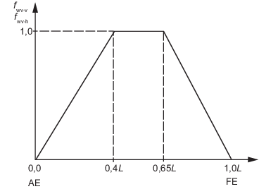
Figure 2.3.1 Vertical and horizontal wave bending moment distribution for scantling
requirements and strength assessment
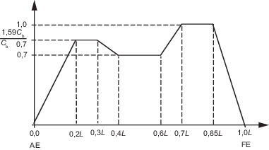
Figure 2.3.2 Positive vertical wave shear force distribution
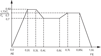
Figure 2.3.3 Negative vertical wave shear force distribution
3.8 Dynamic local loads
3.8.1
General.
- This Section provides the envelope values for dynamic wave
pressure, dynamic tank pressure, green sea load and dynamic deck loads.
- The envelope dynamic wave pressures are given in Pt 10, Ch 2, 3.8 Dynamic local loads 3.8.2.(a).
- The envelope green sea load given in Pt 10, Ch 2, 3.8 Dynamic local loads 3.8.3 only applies to scantling requirements
and strength assessment.
- The envelope dynamic tank pressure is a combination of the
inertial components due to vertical, transverse and longitudinal
acceleration. The envelope dynamic tank pressure components are given in
Pt 10, Ch 2, 3.8 Dynamic local loads 3.8.4.
- The envelope dynamic deck loads are given in Pt 10, Ch 2, 3.8 Dynamic local loads 3.8.5 and Pt 10, Ch 2, 3.8 Dynamic local loads 3.8.6.
3.8.2
Dynamic wave pressure.
- The envelope dynamic wave pressure,
 , is to be taken as the greater of the following: , is to be taken as the greater of the following:
 kNm2 kNm2
 kN/m2 kN/m2
where
-
 = local breadth at the waterline, for considered
draught, not to be taken less than 0,5B, in metres = local breadth at the waterline, for considered
draught, not to be taken less than 0,5B, in metres
-
 = ( = ( + 0,8) + 0,8) 
-
 = =  – – 
 + + 
-
 = 0,25 = 0,25  for |y | < 0,25 for |y | < 0,25
- =
 for |y | ≥ 0,25 for |y | ≥ 0,25
-
 = =  at, and aft of, AE. at, and aft of, AE.
- =
 between 0,2L and 0,7L from AE. between 0,2L and 0,7L from AE.
- =
 + +  at, and forward of, FE. at, and forward of, FE.
intermediate values to be obtained by linear
interpolation
-
 = 1,0 at, and aft of, AE. = 1,0 at, and aft of, AE.
- = 0,7 for 0,2L to 0,7L from AE.
- = 1,0 at, and forward of, FE.
intermediate values to be obtained by linear
interpolation
 , ,  and and  are given in Pt 10, Ch 2, 3.8 Dynamic local loads 3.8.2.(b) for
scantling requirements and strength assessment application. are given in Pt 10, Ch 2, 3.8 Dynamic local loads 3.8.2.(b) for
scantling requirements and strength assessment application.
- For scantling requirements and strength
assessment, the envelope maximum dynamic wave pressure,
 , see
Figure 2.3.4 Transverse
distribution of maximum dynamic wave pressure for scantling
requirements and strength assessment, and minimum dynamic
wave pressure, , see
Figure 2.3.4 Transverse
distribution of maximum dynamic wave pressure for scantling
requirements and strength assessment, and minimum dynamic
wave pressure,  , see
Figure 2.3.5 Transverse
distribution of minimum dynamic wave pressure for scantling
requirements and strength assessment, are to be taken as: , see
Figure 2.3.5 Transverse
distribution of minimum dynamic wave pressure for scantling
requirements and strength assessment, are to be taken as:
 = =  kN/m2 below still waterline kN/m2 below still waterline
=  – 10 (z – – 10 (z –  ) kN/m2 ) kN/m2
for  < z ≤ < z ≤  + + 
= 0 kN/m2 for z >  + + 
 = — = —  kN/m2 below still waterline kN/m2 below still waterline
= 0 kN/m2 above still waterline
where
-
 is not to be taken as less than – is not to be taken as less than –  g (
g ( – z) – z)
where
 = envelope dynamic wave pressure, in
kN/m2, as defined in Pt 10, Ch 2, 3.8 Dynamic local loads 3.8.2.(a) with: = envelope dynamic wave pressure, in
kN/m2, as defined in Pt 10, Ch 2, 3.8 Dynamic local loads 3.8.2.(a) with:
 = heading correction factor, see
Pt 10, Ch 2, 6.3 Application of dynamic loads 6.3.1.(b) = heading correction factor, see
Pt 10, Ch 2, 6.3 Application of dynamic loads 6.3.1.(b)
 = pressure at waterline, to be taken as = pressure at waterline, to be taken as at still waterline, in kN/m2. at still waterline, in kN/m2.
3.8.3
Green sea load.
- The envelope green sea load on the weather deck,
 , is to be taken as the greater of the following: , is to be taken as the greater of the following:
 = =  ( (
 – –  ) kN/m2 ) kN/m2
 = 0,8 = 0,8 ( ( – –  ) kN/m2 ) kN/m2
 = 34,3 kN/m2 = 34,3 kN/m2
where
 = 0,8 + = 0,8 + 
 = 0,5 + = 0,5 + 
 = 1,0 at, and forward of, 0,2L from AE. = 1,0 at, and forward of, 0,2L from AE.
= 0,8 at, and aft of, AE.
intermediate
values to be obtained by linear interpolation
 = =  pressure at still waterline for considered draught,
in kN/m2, see
Pt 10, Ch 2, 3.8 Dynamic local loads 3.8.2.(a) pressure at still waterline for considered draught,
in kN/m2, see
Pt 10, Ch 2, 3.8 Dynamic local loads 3.8.2.(a)
 = =  pressure at still waterline for considered draught,
in kN/m2, see
Pt 10, Ch 2, 3.8 Dynamic local loads 3.8.2.(a) pressure at still waterline for considered draught,
in kN/m2, see
Pt 10, Ch 2, 3.8 Dynamic local loads 3.8.2.(a)
 = distance from the deck to the still waterline at
the applicable draught for the loading condition being considered, in
metres = distance from the deck to the still waterline at
the applicable draught for the loading condition being considered, in
metres
 Bwdk = local breadth at the weather deck, in metres Bwdk = local breadth at the weather deck, in metres
Where loads are available from a model test, they may
be used for design purposes.
3.8.4
Dynamic tank pressure.
- The envelope dynamic tank pressure,
 , due to vertical tank acceleration is to be taken as: , due to vertical tank acceleration is to be taken as:
 = =  kN/m2 for strength assessment and
scantling requirements. kN/m2 for strength assessment and
scantling requirements.
- The envelope dynamic tank pressure,
 , due to transverse acceleration is to be taken as: , due to transverse acceleration is to be taken as:
 = =  kN/m2 for strength assessment and
scantling requirements. kN/m2 for strength assessment and
scantling requirements.
where
 |
= |
factor to account for ullage in cargo tanks, and is
to be taken as: |
| = |
0,67 for cargo tanks, including cargo tanks
designed for filling with water ballast |
| = |
1,0 for ballast and other tanks. |
- The envelope dynamic tank pressure,
 , due to longitudinal acceleration is to be taken as: , due to longitudinal acceleration is to be taken as:
 = = 
 kN/m2 for scantling requirements and
strength assessment kN/m2 for scantling requirements and
strength assessment
where
 |
= |
factor to account for ullage in cargo tanks, and is
to be taken as: |
| = |
0,62 for cargo tanks, including cargo tanks
designed for filling with water ballast |
| = |
1,0 for ballast and other tanks. |
- For scantling requirements and strength
assessment, the simultaneous acting dynamic tank pressure,
 , is to be taken as the summation of the components for
the considered dynamic load case, see
Pt 10, Ch 2, 6.3 Application of dynamic loads 6.3.6. , is to be taken as the summation of the components for
the considered dynamic load case, see
Pt 10, Ch 2, 6.3 Application of dynamic loads 6.3.6.
3.8.5
Dynamic deck pressure from distributed loading.
- The envelope dynamic deck pressure,
 , on decks, inner bottom and hatch covers is to be taken
as: , on decks, inner bottom and hatch covers is to be taken
as:
 = =  kN/m2 kN/m2
where
 = uniformly distributed pressure on lower decks and
decks within superstructure, in kN/m2, as defined in Pt 10, Ch 2, 2.3 Local static loads 2.3.1. = uniformly distributed pressure on lower decks and
decks within superstructure, in kN/m2, as defined in Pt 10, Ch 2, 2.3 Local static loads 2.3.1.
|